EM convergence with varying number of components


(Note: videos below are given in both quicktime and mpeg formats; however, the quicktime videos tend to be higher quality and are therefore recommended. If you do not have quicktime installed, you can download the free player (Mac/Windows) from Apple.)
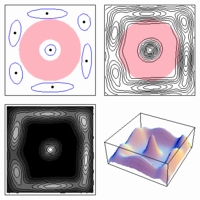
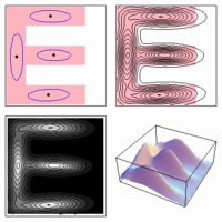
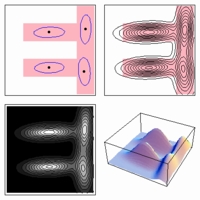
Below, we illustrate EM algorithm convergence for four different 2d synthetic data sets, varying the number of component densities from two to 15. For each animation, the pink region indicates the distribution of the underlying data (uniformly distributed in the pink region), except for the "anti-annular" example, where the white region indicates the data distribution. We also indicate the log-likelihood of test data given the estimated parameter values as a function of the number of component densities. Note how the test data log-likelihood levels out after a sufficient number of component densities are included in the mixture model.
Annular region
(400 x 400)


Log-likelihood vs. num. of component densities
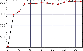

(high-quality, quicktime, 1 Mb)

(lower-quality, mpeg, 880 kb)
Anti-annular region
(400 x 400)


Log-likelihood vs. num. of component densities
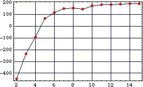

(high-quality, quicktime, 1.2 Mb)

(lower-quality, mpeg, 1 Mb)
E-shaped polygonal region
(400 x 400)


Log-likelihood vs. num. of component densities
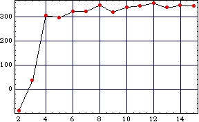

(high-quality, quicktime, 1 Mb)

(lower-quality, mpeg, 1 Mb)
Anti E-shaped polygonal region
(400 x 400)


Log-likelihood vs. num. of component densities
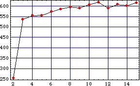

(high-quality, quicktime, 1 Mb)

(lower-quality, mpeg, 948 kb)

Last updated Spetember 8, 2003 by Michael C. Nechyba