Detailed Mixture-Model Examples


(Note: videos below are given in both quicktime and mpeg formats; however, the quicktime videos tend to be higher quality and are therefore recommended. If you do not have quicktime installed, you can download the free player (Mac/Windows) from Apple.)
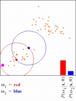
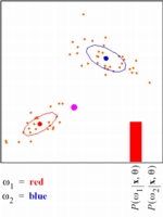
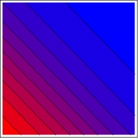
Below we illustrate a detailed, two-component mixture model experiment, where we illustrate the posterior probability for each component and data point. The first animation illustrates the posterior probability for the initial parameter values of the mixture model; the second animation illustrates the posterior probability for the final parameter values of the mixture model after the EM algorithm has converged; finally, the last animation illustrates the posterior probability over the entire region of interest for each component as a function of EM algorithm iterations. In each plot, red denotes the first component of the mixture model, while blue denotes the second component of the mixture model.
Posterior probabilities for initial parameter values
(288 x 384)

(The pink dot in the animations indicates the data point for which the posterior probabilities are plotted in the bottom right-hand corner of the plot.)

(high-quality, quicktime, 1 Mb)

(lower-quality, mpeg, 188 kb)
Posterior probabilities for final parameter values
(288 x 384)

(The pink dot in the animations indicates the data point for which the posterior probabilities are plotted in the bottom right-hand corner of the plot.)

(high-quality, quicktime, 984 kb)

(lower-quality, mpeg, 156 kb)
Posterior probabilities over the entire region as a function of EM iterations
(288 x 288)


(high-quality, quicktime, 140 kb)

(lower-quality, mpeg, 72 kb)

Last updated Spetember 8, 2003 by Michael C. Nechyba