Section 1: Two-link planar manipulator
DH parameters
![]()
![]()
Numeric values for simulation
![]()
![]()
Nonsingular inverse Jacobian trajectory
This section simulates the relationship ![]() for a non-singular, circular, end-effector trajectory.
for a non-singular, circular, end-effector trajectory.
![RowBox[{RowBox[{pick = {1, 1} ;, , (* select first two rows of Jacobian *), <br />, RowBox[{R ... } // N ;, , (* initial joint angles *), <br />, maxTime = 2Pi // N ;}], (* simulation length *)}]](../HTMLFiles/index_14.gif)
![]()
![]()
![]()
![[Graphics:../anim1.gif]](../anim1.gif)
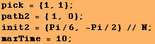
Singular inverse Jacobian trajectory
This section simulates the relationship ![]() for a straight-line end-effector trajectory that results in a singularity.
for a straight-line end-effector trajectory that results in a singularity.
![]()
![]()
![]()
![]()
![[Graphics:../anim2.gif]](../anim2.gif)
Joint velocities ![]()
![]()
![]()
![]()
![]()
![[Graphics:../HTMLFiles/index_73.gif]](../HTMLFiles/index_73.gif)
Created by Mathematica (October 1, 2003)